
Using Compressive Sensing to Recover Lotka-Volterra Dynamics
Compressive Sensing 101
Compressive sensing (also known as compressed sensing) is a method used to solve sparse, underdetermined matrix systems which was developped around 2004. Let's unpack that sentence with an example. $$ \begin{align*} 2x + y &= 5\\ 2x + y + z &=8 \end{align*} $$ In this system of equations, we have 3 unknowns and 2 equations, so the system is underdetermined: there are more unknowns than equations. This poses a problem for traditional solving techniques because, as you might recall, you need at least the same number of independent equations as you have variables. In this case, we can quickly check that this is indeed true. We obtain a family of solutions, or a set of multiple solutions. We know that $ z=3 $, but any combination of $ x, y $ works, so long as $ 2x +y = 5 $. Another way of stating this is that any point on the line $ y=-2x+5 $ solves the system. If this system was all the information we had, we'd be at a standstill. However, we have one more condition: sparsity. All sparsity says is that a significant number of the variables have a value of zero. How many? No idea. Which ones? We don't know. Even still, with this condition of sparsity, we can solve this underdetermined matrix system(1). Just as a refresher, the above system can be written in the following way using matrices. $$ \begin{pmatrix} 2 & 1 & 0\\ 2 & 1 & 1 \end{pmatrix} \times \begin{pmatrix} x\\ y\\ z \end{pmatrix} = \begin{pmatrix} 5\\ 8 \end{pmatrix} $$ So how do we (or a computer) pick a sparse solution from the sample space of possible solutions? For that, we turn to measure theory. Measure theory is a branch of mathematics that concerns itself with ways we can measure real things and mathematical objects, the properties of measures, and why all of that matters in the first place. Say you're handed a box and given the instructions "measure it". A very reasonable first question would be how? Do you want the volume? The height? The surface area? The mass? We'd pick a measure depending on why we want to measure the box. If we're trying to paint it, we'd pick surface area. If we want to see if it would fit under my bed, we'd pick height, etc.Just as we can measure real things, like a box, in different ways, we can also measure a solution to our system. Recall that any point on the line $ y=-2x+5 $ is a solution, so when I say a solution, I mean a point on that line such as $(2, 1)$ or $(-1, 7)$. Now, if we wanted to "measure" the point $(2, 1)$ we could use the sum of the absolute values of the $x$ and $y$ variables to obtain a value of $2+1=3$. This method is called the $\ell_1$ norm (2). We could also measure it by its distance to the origin, or the Euclidean norm, by taking $\sqrt{x^2+y^2}=\sqrt{4+1}=\sqrt{5}$. This way of measuring is called the $\ell_2$ norm. Now, like two different boxes might have the same value by a given measure (like the same volume), but be different sizes, different points also can have the same value under a given norm. For example, $(0,1)$, $(1,0)$, $(0.75,-0.25)$, and $(-0.5, -0.5)$ all have the same $\ell_1$ norm.
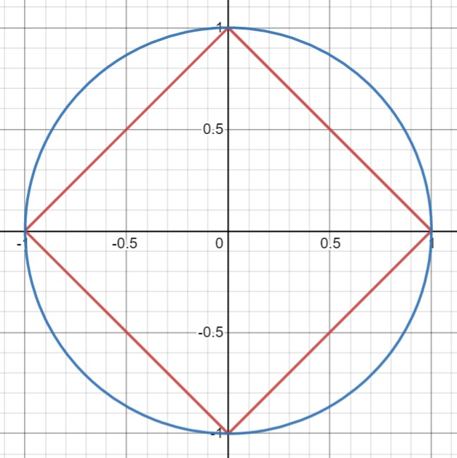
Figure 1: The unit ball of the $\ell_1$ (in red) and $\ell_2$ norms (in blue). The unit "ball" is all the points that have a value of 1 for a given norm. Yes, it is called a unit ball even when it is very pointy.
In the $\ell_1$ norm, all of the points with the same value make a diamond shape, and in the $\ell_2$ norm, all of the points with the same value make a circle (both of which are centred at 0), as we can see in the image above.
Now, why we took that digression into measure theory is because of the way compressive sensing chooses one answer from a whole sample space of answers. The final answer given is the answer in the sample space with the smallest $\ell_1$ norm. When we find the smallest solution in the $\ell_1$ norm, we are, in effect, asking what is the smallest diamond that touches the line of solutions, and where on the line do they touch? Because of the diamond shape of the unit ball in the $\ell_1$ norm, the smallest diamond that touches the sample space will almost certainly touch the line at one of its points. Its points also happen to be on the axes, which means that at least one of the variables is 0. We can compare this to the $\ell_2$ norm again. The smallest circle by contrast, does not intersect the sample space along an axis, and therefore does not give a sparse solution.
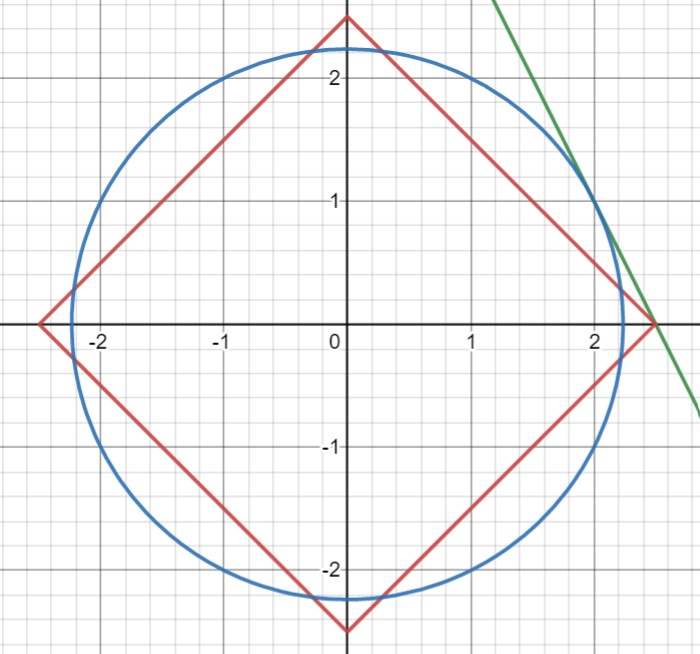
Figure 2: The points with the minimum $\ell_1$ (in red) and $\ell_2$ norm values in our sample space (in green).
This extends into even higher dimensions. In three dimensions, we would have a plane of solutions instead of a line, and the unit "ball" in $\ell_1$, instead of being a diamond, would be a tetrahedron. In 4D and up, it gets impossible to visualize, but the math still holds.
This technique has a lot of uses outside of ecology. As you can imagine, the idea of recovering the more information with fewer equations or samples has obvious applications in information theory: the science of how we store, compress, and restore information.
The Ecology Connection
One of the key questions in ecology is how populations of various species will change and affect each other over time. One of the oldest and most common ways of representing these relations is the Lotka-Volterra equations, which are pairs of first-order nonlinear differentiable equations. $$ \begin{align*} \frac{dx}{dt}&=\alpha x - \beta xy\\ \frac{dy}{dt}&=\delta xy - \gamma y \end{align*} $$ All the above Lotka-Volterra equations say is that the rate of change of species $x$, the prey, is determined by how fast the prey population would grow if left to its own devices (the $\alpha x$ term), subtracted by the rate of predation, which depends on the current level of predator and prey populations (the $\beta xy$ term). By contrast, the rate that the predator population increases depends on how much prey they catch (the $\delta xy$ term) and decreases in the absence of the prey species (the $\gamma y$ term). The spirit of my project is whether or not compressive sensing is useful to figure out the values of $\alpha, \beta,\delta,\gamma$. In a real ecosystem model, we'd have two unknown variables for every single pair of species, one term for the effect each species has on every other species. This is lots of variables, but it is a sound assumption that the matrix of all these coefficients is sparse, as most species don't really affect each other unless they are directly in competition or have a predator-prey relationship.The nature of the data is difficult to deal with, as often ecologists are not lucky enough to have population data for all species, and not over long periods of time either. As such, techniques like compressive sensing are incredibly promising because they require fewer input datapoints/equations to predict the coefficients and therefore the ecosystem. My research mostly concerns how we can massage ecological data into a form that we can use compressive sensing on and how efficient it is at recovering the underlying dynamics (the coefficients and equations) using only population data.
I thought it was a pretty neat project. I hope you do too. Thanks for reading to all the way down here.
(1) The exceptionally keen ones of you out there might say: but wait, we could just solve this equation by hand now that we know that $ x $ or $ y $ is $ 0 $, and you're right, it's quite trivial in this toy example. However, less trivial when you're working with hundreds of variables, and you have no idea which ones or how many are zero. The example is merely to illustrate the technique and unfortunately isn't a perfect showcase of the power of compressive sensing. Bear with me, it gets more exciting soon.
(2) I've skipped over a lot of (all of) the nuance of norms and measures. They are different. Forgive me analysis gods.